Chambolle-Pock-Bregman
This document is devoted to the resolution of discrete mean field games via Chambolle-Pock-Bregman algorithm (see [CP16]). We investigate proximity operators beased on the Kullback-Leibler divergence to compute running cost step.
We define \(\mathcal{T} = \{0,\ldots,T-1\}\), \(\bar{\mathcal{T}} = \{0,\ldots,T\}\) and \(S=\{0,\ldots,n\}\). We set \(\Delta_t = 1/T\) and \(\Delta_x = 1/n\). Let \(\xi\) be a 1-strongly convex function. For any \(m_1,m_2 \in \mathbb{R}(S)\) we define the Bregman divergence
We define the associated generalized proximity operator
Note that if \(D(m_1,m_2) = \|m_1-m_2\|_m^2\) then we are in the classical proximal case. For any \(m_1, m_2 \in \Delta(S)/\Delta_x\), we define the Kullback-Leibler divergence
which is equivalent to
Strong convexity
For any \(\Delta_x m_1, \Delta_x m_2 \in \Delta(S)\),
thus we deduce that \( \sum_{t \in \mathcal{T}}\Delta_t h[\cdot](t) + h[\cdot](T)\) is 1-strongly convex with respect to \(\|\cdot\|_m.\)
Packages
import numpy as np
from numpy import random
from mpl_toolkits import mplot3d
import matplotlib
import matplotlib.pyplot as plt
import matplotlib.animation as animation
import time
Algorithms
The Bregman-Chambolle-Pock algorithm is a primal-dual method which aims at finding a saddle-point in optimization problems of the following form:
for any \(K\) bounded operator, \(F\) and \(G\) l.s.c. convex and proper functions, \(H\) with Lipschitz gradient.
Non-linear primal dual algorithm
Let \(D_x\) and \(D_y\) two distances, the algorithm is given by
find
find
update
Remark
If \(D_x\) and \(D_y\) are euclidean norms then \(x^{n+1}\) and \(y^{n+1}\) can be written:
update
find
We define
In our case, we have the following saddle point problem:
where
Notice that depending on the assumptions on \(F\) and \(\phi\), one could identify \(\mathcal{F}_2\) either with \(f\) or \(g\) in the abstract algorithm above.
The algorithm is given by:
find
find
update
Data of the problem
def initial_mass(n):
    m_bar = np.zeros(n)
    for x in range(n):
        m_bar[x] = np.exp(-(x-n/2)**2/(n/4)**2)
    return(n*m_bar/np.sum(m_bar))


def displacement_cost(T,n):
    dx=1/n
    dt=1/T
    disp = np.zeros((T-1,n,n))
    for t in range(T-1):
        for x in range(n):
            for y in range(n):
                disp[t,x,y] = ((y-x)*dx/dt)**2/4
    return(disp)

def penalisation_congestion(T,n):
    nu = np.zeros((T,n))
    for t in range(T):
        if t > T/2 and t < 3*T/4:
            for x in range(n):
                if x > n/2:
                    nu[t,x] = 10
    return(nu)

def sharp_penalisation_congestion(T,n):
    eta = np.zeros((T,n)) + 3
    for t in range(T):
        for x in range(n):
            if (t > T/3 and t < 2*T/3) and (x > n/3 and x < 2*n/3):
                    eta[t,x] = 1/4
    return(eta)

def reference_demand(T):
    new_D_bar = np.zeros(T-1)
    for t in range(T-1):
        new_D_bar[t] = np.sin(t*(4*np.pi)/(T-1))
    return(new_D_bar)

def alpha_cost(T,n):
    dx=1/n
    dt=1/T
    disp = np.zeros((T-1,n,n))
    for t in range(T-1):
        for x in range(n):
            for y in range(n):
                disp[t,x,y] = (y-x)*dx/dt
    return(disp)
Computation of Chambolle-Pock steps
Computation of \((P^{n+1},u^{n+1},\gamma^{n+1})\)
For any \((k_1,k_2,k_3) \in \mathcal{K}\) we have that
Then we have that
def prox_P(P,D,w,T,n,sigma,alpha):
    dx=1/n
    return(P + sigma*(np.sum(alpha*w*dx)-D))
Computation of \(u^{n+1}\)
def prox_u(u,m_1,w,m_0,sigma,T,n):
    dt=1/T
    new_u = np.zeros((T,n))
    for t in range(T):
        if t==0:
            new_u[t] = u[t] + sigma*(m_0-m_1[t])
        else:
            for x in range(n):
                new_u[t,x] = u[t,x] + sigma*(np.sum(w[t-1,:,x]) - m_1[t,x])/dt
    return new_u
Computation of \(\gamma^{n+1}\)
def prox_gamma(gamma,m_1,m_2,sigma):
    return(gamma + sigma*(m_1-m_2))
Computation of \((m_1^{n+1},m_2^{n+1},w^{n+1},D^{n+1})\)
We recall that
Then we have
\((m_1^{n+1},w^{n+1})\) is given by
\(m_2^{n+1}\) is given by
\(D^{n+1}\) is given by
Computation of \(D^{n+1}\)
We have that
def prox_phi_star_quad(X,Db,D_0,tau,T,n,D_min,D_max):
    argmin = (X - tau*D_0*Db)/(1 + tau*D_0)
    if argmin > D_max:
        argmin = D_max
    if argmin < D_min:
        argmin = D_min
    return(argmin)

def Local_D_prox_quad(D,P,T,n,tau,Db,D_0,D_min,D_max):
    c= D + tau*P
    new_Dt = prox_phi_star_quad(c,Db,D_0,tau,T,n,D_min,D_max)
    return(new_Dt)

def D_prox_quad(D,P,T,n,tau,alpha,Db,D_0,D_min,D_max):
    new_D = np.zeros(T-1)
    for t in range(T-1):
        new_D[t] = Local_D_prox_quad(D[t],P[t],T,n,tau,Db[t],D_0,D_min,D_max)
    return new_D
Computation of \(m_2^{n+1}\)
def prox_coeff_F_sharp(X,nu,eta,coeff,T,n):
    argmin = (X - coeff*nu)/(coeff + 1)
    if argmin>eta:
        argmin = eta
    if argmin<0:
        argmin = 0
    return(argmin)

def m_2_prox(m_2,gamma,nu,eta,tau,T,n):
    m_2_new = np.zeros((T,n))
    c_2 = 0
    for t in range(T):
        for x in range(n):
            c_2 = m_2[t,x] + tau*gamma[t,x]
            m_2_new[t,x] = prox_coeff_F_sharp(c_2,nu[t,x],eta[t,x],tau,T,n)
    return(m_2_new)
Computation of \((m_1^{n+1},w^{n+1})\)
For any \(t \in \mathcal{T}\), we have that
where
To solve this problem we form the following Lagrangian
For any \((t,x,y) \in \mathcal{T} \times S \times S\), the first order conditions lead to the following system
To simplify the notations we define \(\tilde{a} = \exp{a}\), \(\hat{m}_1^n = m_1^n/\tilde{c}_1\) and \(\hat{w}^n = w^n/\tilde{c}_3\). Then the two first equations of the above system can be written
we denote \(\hat{m}_1^n = m_1^n/\tilde{c}_1\) and \(\hat{w}^n = w^n/\tilde{c}_3\), thus
If \(\lambda_2(t,x) > 0\), the last two inequalities of the system of four equations lead to
then we have that
Thus we deduce that
If \(\lambda_2(t,x) = 0\), then we have
and
For \(t=T\), the first order conditions lead
If \(\lambda_2(t,x) > 0\), we have that
If \(\lambda_2(t,x) = 0\), we have that
def m_1_w_proj(P,gamma,u,m_1,w,T,n,tau,alpha,beta):
    dt = 1/T
    dx=1/n
    (new_m_1,new_w) = (np.zeros((T,n)),np.zeros((T-1,n,n)))
    c_1 = np.zeros((T,n))
    c_3 = np.zeros((T-1,n,n))
    m_hat = np.zeros((T,n))
    w_hat = np.zeros((T-1,n,n))
    sum_w_hat = np.zeros((T-1,n))
    tilde_lambda_1 = 0
    tilde_lambda_2 = 0
    for t in range(T-1):
        for x in range(n):
            c_1[t,x] = tau*(-u[t,x]/dt + gamma[t,x])
            c_3[t,x] = tau*(beta[t,x] + alpha[t,x]*P[t] + u[t+1]/dt)
            m_hat[t,x] = m_1[t,x]/np.exp(c_1[t,x])
            w_hat[t,x] = w[t,x]/np.exp(c_3[t,x])
            sum_w_hat[t,x] = np.sum(w_hat[t,x])
            tilde_lambda_2 = m_hat[t,x]*sum_w_hat[t,x]/(dx**2)
            tilde_lambda_1 = 1/(dx*sum_w_hat[t,x])
            new_m_1[t,x] = 1/dx
            new_w[t,x] = w_hat[t,x]*tilde_lambda_1
            if tilde_lambda_2 <= 1:
                tilde_lambda_1 = np.sqrt(m_hat[t,x]/sum_w_hat[t,x])
                new_w[t,x] = w_hat[t,x]*tilde_lambda_1
                new_m_1[t,x] = m_hat[t,x]/(tilde_lambda_1)
    for x in range(n):
        c_1[T-1,x] = tau*(-u[T-1,x] + gamma[T-1,x])
        m_hat[T-1,x] = m_1[T-1,x]/np.exp(c_1[T-1,x])
        tilde_lambda_2 = dx*m_hat[T-1,x]
        new_m_1[T-1,x] = 1/dx
        if tilde_lambda_2 <= 1:
            new_m_1[T-1,x] = m_hat[T-1,x]
    return (new_m_1,new_w)
Computation of \((\bar{m}_1^{n+1},\bar{m}_2^{n+1},\bar{w}^{n+1},\bar{D}^{n+1})\)
def relax(var_m_1,var_m_2,var_w,var_D,m_1,m_2,w,D,theta):
    m_1_bar = var_m_1 + theta*(var_m_1-m_1)
    m_2_bar = var_m_2 + theta*(var_m_2-m_2)
    w_bar = var_w + theta*(var_w-w)
    D_bar = var_D + theta*(var_D-D)
    return(m_1_bar,m_2_bar,w_bar,D_bar)
def ergodic(var_m_1,var_m_2,var_w,var_D,var_u,var_gamma,var_P,m_1,m_2,w,D,u,gamma,P,k):
    m_1_bar = var_m_1/(k+1) + k*m_1/(k+1)
    m_2_bar = var_m_2/(k+1) + k*m_2/(k+1)
    w_bar = var_w/(k+1) + k*w/(k+1)
    D_bar = var_D/(k+1) + k*D/(k+1)
    u_bar = var_u/(k+1) + k*u/(k+1)
    gamma_bar = var_gamma/(k+1) + k*gamma/(k+1)
    P_bar = var_P/(k+1) + k*P/(k+1)
    return(m_1_bar,m_2_bar,w_bar,D_bar,u_bar,gamma_bar,P_bar)
Strategy \(\pi = w/m\) and average strategy
def equilibrium_strategy(m,w,T,n,tol=1e-5):
    strat = np.zeros((T-1,n,n))
    for t in range(T-1):
        for x in range(n):
            if m[t,x] > tol:
                strat[t,x] = w[t,x]/m[t,x]
    return(strat)

def mean_field_strategy(pi,T,n):
    mfs = np.zeros((T-1,n))
    for t in range(T-1):
        for x in range(n):
            for y in range(n):
                mfs[t,x] += pi[t,x,y]*(y-x)
    return(mfs)
Reconstruction of \((u,\pi[u])\)
def d_p_mapping(m,w,gamma,P,alpha,beta,T,n,tol = 1e-3,mfg=1):
    dt=1/T
    dx=1/n
    new_u = np.zeros((T,n))
    new_pi = np.zeros((T-1,n,n))
    f = np.zeros((T,n))
    if mfg == 1:
        f = gamma
    new_u[T-1] = f[T-1]
    for t in range(T-1):
        for x in range(n):
            cost = np.zeros(n)
            cost = beta[T-2-t,x]*dt + alpha[T-2-t,x]*P[T-2-t]*dt + new_u[T-1-t]
            argmin = np.argmin(cost)
            if m[T-2-t,x]*dx>tol:
                new_pi[T-2-t,x] = w[T-2-t,x]/m[T-2-t,x]
            else:
                new_pi[T-2-t,x,argmin] = 1
            new_u[T-2-t,x] = cost[argmin] + f[T-2-t,x]*dt
    return(new_u,new_pi)
Computation of \(\|\mathcal{A}\|\)
A key condition in the Chambolle-Pock algorithm is given by \( \sigma \tau L^2 < 1\) where \(L = \|\mathcal{A}\|\). For any \((m_1,m_2,w,D) \in \hat{\mathcal{K}}\) we have that
where
Thus
Finally
def norm_A(alpha,n,T):
    dt=1/T
    dx = 1/n
    norm_alpha = 0
    for x in range(n):
        norm_alpha = norm_alpha + np.sum(alpha[0,x]**2)
    return(np.sqrt(2*(n/(dt**2) + norm_alpha)))
Error function
def verification(P,u,gamma,m,pi,w,T,n,beta,nu,m_0,alpha,Db,Dmin,Dmax,eta,mfg = 1):
    cost = np.zeros((T-1,n))
    Delta_u = np.zeros((T,n))
    Delta_pi = np.zeros((T-1,n,n))
    Delta_m = np.zeros((T,n))
    Delta_gamma = np.zeros((T,n))
    Delta_P = np.zeros(T-1)
    demand = np.zeros((T-1,n,n))
    dt=1/T
    dx=1/n
    f = np.zeros((T,n))
    if mfg == 1:
        f = gamma
    Delta_m[0] = abs(m[0] - m_0)*dx
    for x in range(n):
        Delta_u[T-1,x] = abs(u[T-1,x] - f[T-1,x])*dx
    for t in range(T-1):
        for x in range(n):
            arg = beta[t,x]*dt + alpha[t,x]*P[t]*dt + u[t+1]
            demand[t,x] = pi[t,x]*m[t,x]*alpha[t,x]*dx
            cost[t,x] = np.sum(pi[t,x]*(beta[t,x]*dt + alpha[t,x]*P[t]*dt)) + f[t,x]*dt
            Delta_pi[t,x] = abs(np.sum(pi[t,x]*arg) - np.sort(arg)[0])*dx
            Delta_m[t+1,x] = abs(m[t+1,x] - np.sum(pi[t,:,x]*m[t]))*dx
            Delta_u[t,x] = abs(u[t,x] - cost[t,x] - np.sum(pi[t,x]*u[t+1]))*dx
            if gamma[t,x] < nu[t,x]:
                Delta_gamma[t,x] = abs(gamma[t,x])*dt*dx
            elif gamma[t,x] > eta[t,x] + nu[t,x]:
                Delta_gamma[t,x] = abs(gamma[t,x] - eta[t,x])*dt*dx
            else:
                Delta_gamma[t,x] = abs(gamma[t,x] - m[t,x] - nu[t,x])*dt*dx
        D = np.sum(demand[t])
        if P[t] > D_0*(Db[t]+Dmax):
            Delta_P[t] = abs(P[t]-D_0*(Db[t]+Dmax))*dt
        elif P[t] < D_0*(Db[t]+Dmin):
            Delta_P[t] = abs(P[t]-D_0*(Db[t]+Dmin))*dt
        else:
            Delta_P[t] = abs(P[t]- D_0*(Db[t]+D))*dt
    return (np.sum(Delta_u),np.sum(Delta_pi),np.sum(Delta_m),np.sum(Delta_P),np.sum(Delta_gamma))
Local transition version
tran_0 = np.array([0,1])
tran_interm = np.array([-1,0,1])
tran_n = np.array([-1,0])

def tran(x,n):
    if x == 0:
        return(tran_0)
    if x == n-1:
        return(tran_n)
    else:
        return(tran_interm)

def norm_A(alpha,n,T):
    dt=1/T
    norm_alpha = 0
    cst = 0
    for x in range(n):
        Y = tran(x,n) + x
        norm_alpha = norm_alpha + np.sum(alpha[0,x,Y]**2)
        if len(Y)>cst:
            cst = len(Y)
    return(np.sqrt(2*(cst/(dt**2) + norm_alpha)))

def equilibrium_strategy(m,w,T,n,tol=1e-2):
    strat = np.zeros((T-1,n,n))
    for t in range(T-1):
        for x in range(n):
            Y = tran(x,n) + x
            if m[t,x] > tol:
                strat[t,x,Y] = w[t,x,Y]/m[t,x]
    return(strat)

def m_1_w_proj(P,gamma,u,m_1,w,T,n,tau,alpha,beta):
    dt = 1/T
    dx=1/n
    (new_m_1,new_w) = (np.zeros((T,n)),np.zeros((T-1,n,n)))
    c_1 = np.zeros((T,n))
    c_3 = np.zeros((T-1,n,n))
    m_hat = np.zeros((T,n))
    w_hat = np.zeros((T-1,n,n))
    sum_w_hat = np.zeros((T-1,n))
    tilde_lambda_1 = 0
    tilde_lambda_2 = 0
    for t in range(T-1):
        for x in range(n):
            Y = tran(x,n) + x
            c_1[t,x] = tau*(-u[t,x]/dt + gamma[t,x])
            c_3[t,x,Y] = tau*(beta[t,x,Y] + alpha[t,x,Y]*P[t] + u[t+1,Y]/dt)
            m_hat[t,x] = m_1[t,x]/np.exp(c_1[t,x])
            w_hat[t,x,Y] = w[t,x,Y]/np.exp(c_3[t,x,Y])
            sum_w_hat[t,x] = np.sum(w_hat[t,x,Y])
            tilde_lambda_2 = m_hat[t,x]*sum_w_hat[t,x]*dx**2
            tilde_lambda_1 = 1/(dx*sum_w_hat[t,x])
            new_m_1[t,x] = 1/dx
            new_w[t,x,Y] = w_hat[t,x,Y]*tilde_lambda_1
            if tilde_lambda_2 <= 1:
                tilde_lambda_1 = np.sqrt(m_hat[t,x]/sum_w_hat[t,x])
                new_w[t,x,Y] = w_hat[t,x,Y]*tilde_lambda_1
                new_m_1[t,x] = m_hat[t,x]/tilde_lambda_1
    for x in range(n):
        c_1[T-1,x] = tau*(-u[T-1,x] + gamma[T-1,x])
        m_hat[T-1,x] = m_1[T-1,x]/np.exp(c_1[T-1,x])
        tilde_lambda_2 = dx*m_hat[T-1,x]
        new_m_1[T-1,x] = 1/dx
        if tilde_lambda_2 <= 1:
            new_m_1[T-1,x] = m_hat[T-1,x]
    return (new_m_1,new_w)

def prox_P(P,D,w,T,n,sigma,alpha):
    dx=1/n
    new_P = np.zeros(T-1)
    for t in range(T-1):
        result = 0
        for x in range(n):
            Y = tran(x,n) + x
            result += np.sum(alpha[t,x,Y]*w[t,x,Y])
        new_P[t] = P[t] + sigma*(result*dx - D[t])
    return new_P


def prox_u_dualnorm(u,m_1,w,m_0,sigma,T,n):
    dt=1/T
    dx=1/n
    new_u = np.zeros((T,n))
    for t in range(T):
        if t==0:
            #print(u[t,0],sigma*(m_0[0]-m_1[t,0]))
            new_u[t] = np.log(np.exp(u[t]) + sigma*(m_0-m_1[t]))
        else:
            for x in range(n):
                Y = tran(x,n) + x
                new_u[t,x] = np.log(np.exp(u[t,x]) + sigma*(np.sum(w[t-1,Y,x]) - m_1[t,x])/dt)
    return new_u

def prox_u(u,m_1,w,m_0,sigma,T,n):
    dt=1/T
    dx=1/n
    new_u = np.zeros((T,n))
    for t in range(T):
        if t==0:
            new_u[t] = u[t] + sigma*(m_0-m_1[t])
        else:
            for x in range(n):
                Y = tran(x,n) + x
                new_u[t,x] = u[t,x] + sigma*(np.sum(w[t-1,Y,x]) - m_1[t,x])/dt
    return new_u

def d_p_mapping(m,w,gamma,P,alpha,beta,T,n,tol = 1e-3,mfg=1):
    dt=1/T
    dx=1/n
    new_u = np.zeros((T,n))
    new_pi = np.zeros((T-1,n,n))
    f = np.zeros((T,n))
    if mfg == 1:
        f = gamma
    new_u[T-1] = f[T-1]
    for t in range(T-1):
        for x in range(n):
            cost = np.zeros(n)
            Y = tran(x,n) + x
            cost[Y] = beta[T-2-t,x,Y]*dt + alpha[T-2-t,x,Y]*P[T-2-t]*dt + new_u[T-1-t,Y]
            argmin = np.argmin(cost[Y])
            if m[T-2-t,x]*dx>tol:
                new_pi[T-2-t,x,Y] = w[T-2-t,x,Y]/m[T-2-t,x]
            else:
                new_pi[T-2-t,x,Y[argmin]] = 1
            new_u[T-2-t,x] = cost[Y[argmin]] + f[T-2-t,x]*dt
    return(new_u,new_pi)

def verification(P,u,gamma,m,pi,w,T,n,beta,nu,m_0,alpha,Db,Dmin,Dmax,eta,mfg = 1):
    cost = np.zeros((T-1,n))
    Delta_u = np.zeros((T,n))
    Delta_pi = np.zeros((T-1,n,n))
    Delta_m = np.zeros((T,n))
    Delta_gamma = np.zeros((T,n))
    Delta_P = np.zeros(T-1)
    demand = np.zeros((T-1,n,n))
    dt=1/T
    dx=1/n
    f = np.zeros((T,n))
    if mfg == 1:
        f = gamma
    Delta_m[0] = abs(m[0] - m_0)*dx
    for x in range(n):
        Delta_u[T-1,x] = abs(u[T-1,x] - f[T-1,x])*dx
    for t in range(T-1):
        for x in range(n):
            Y = tran(x,n) + x
            arg = beta[t,x,Y]*dt + alpha[t,x,Y]*P[t]*dt + u[t+1,Y]
            demand[t,x,Y] = pi[t,x,Y]*m[t,x]*alpha[t,x,Y]*dx
            cost[t,x] = np.sum(pi[t,x,Y]*(beta[t,x,Y]*dt + alpha[t,x,Y]*P[t]*dt)) + f[t,x]*dt
            Delta_pi[t,x] = abs(np.sum(pi[t,x,Y]*arg) - np.sort(arg)[0])*dx
            Delta_m[t+1,x] = abs(m[t+1,x] - np.sum(pi[t,Y,x]*m[t,Y]))*dx
            Delta_u[t,x] = abs(u[t,x] - cost[t,x] - np.sum(pi[t,x,Y]*u[t+1,Y]))*dx
            if gamma[t,x] < 0:
                Delta_gamma[t,x] = abs(m[t,x])*dt*dx
            elif gamma[t,x] > eta[t,x] + nu[t,x]:
                Delta_gamma[t,x] = abs(m[t,x] - eta[t,x])*dt*dx
            else:
                Delta_gamma[t,x] = abs(gamma[t,x] - m[t,x])*dt*dx
        D = np.sum(demand[t])
        if P[t] > D_0*(Db[t]+Dmax):
            Delta_P[t] = abs(D-Dmax)*dt
        elif P[t] < D_0*(Db[t]+Dmin):
            Delta_P[t] = abs(D-Dmin)*dt
        else:
            Delta_P[t] = abs(D- (P[t]/D_0 - Db[t]))*dt
    return (np.sum(Delta_u),np.sum(Delta_pi),np.sum(Delta_m),np.sum(Delta_P),np.sum(Delta_gamma))
Classical Chambolle-Pock
MFG
T = 50
n = 50

alpha = np.zeros((T-1,n,n))

Dmin = -10
Dmax = 10

L = norm_A(alpha,n,T) + 1
sigma = 1/L
tau = 1/L
theta = 1


beta = displacement_cost(T,n)
#nu = penalisation_congestion(T,n)
nu = np.zeros((T,n))
eta = sharp_penalisation_congestion(T,n)

D_0 = 1
Db = np.zeros(T-1)
m_0 = initial_mass(n)

var_m_1 = np.zeros((T,n)) + 1
var_m_2 = var_m_1
var_w = np.zeros((T-1,n,n)) + 1/n
D = np.zeros(T-1)
var_D = D


P = np.zeros(T-1)
u = np.zeros((T,n)) + 1
gamma = np.zeros((T,n))

(m_1_bar,m_2_bar,w_bar,D_bar) = (var_m_1,var_m_2,var_w,var_D)

(av_m_1,av_m_2,av_w,av_D,av_u,av_gamma,av_P) = (m_1_bar,m_2_bar,w_bar,D_bar,u,gamma,P)

N = 10000
start = time.time()
mfg_error = np.zeros((N,5))
ev_m_s = np.zeros((N,T-1,n))
ev_m = np.zeros((N,T,n))
ev_u = np.zeros((N,T,n))

start = time.time()
for i in range(N):
    print(round(i/N*100, 2),"              \r",end = '')

    #P = prox_P(P,D_bar,w_bar,n,alpha)
    u = prox_u(u,m_1_bar,w_bar,m_0,sigma,T,n)
    gamma = prox_gamma(gamma,m_1_bar,m_2_bar,sigma)
    (m_1,m_2,w,D) = (var_m_1,var_m_2,var_w,var_D)
    #var_D = D_prox_quad(D,P,T,n,tau,alpha,D_bar,D_0)
    var_m_2 = m_2_prox(m_2,gamma,nu,eta,tau,T,n)
    (var_m_1,var_w) = m_1_w_proj(P,gamma,u,m_1,w,T,n,tau,alpha,beta)
    (m_1_bar,m_2_bar,w_bar,D_bar) = relax(var_m_1,var_m_2,var_w,var_D,m_1,m_2,w,D,theta)

    (av_m_1,av_m_2,av_w,av_D,av_u,av_gamma,av_P) = ergodic(var_m_1,var_m_2,var_w,var_D,u,gamma,P,av_m_1,av_m_2,av_w,av_D,av_u,av_gamma,av_P,i)
    (U,Pi) = d_p_mapping(av_m_1,av_w,av_gamma,av_P,alpha,beta,T,n,tol = 1e-4)
    mfg_error[i] = np.array(verification(av_P,U,av_gamma,av_m_1,Pi,av_w,T,n,beta,nu,m_0,alpha,Db,Dmin,Dmax,eta))
    (ev_m_s[i],ev_m[i],ev_u[i]) = (mean_field_strategy(Pi,T,n),av_m_1,U)
    end = time.time()

print("\n execution time :",round(end-start,2), "s")
99.99
 execution time : 4108.03 s
#plt.plot(np.log(mfg_error[:,0])/np.log(10), label = r'$\log(||\varepsilon_u||_1)$', color = 'blue')
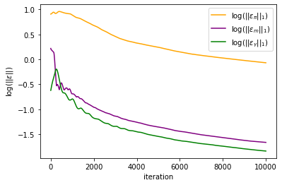
plt.plot(np.log(mfg_error[:,1])/np.log(10), label = r'$\log(||\varepsilon_\pi||_1)$', color = 'orange')
plt.plot(np.log(mfg_error[:,2])/np.log(10), label = r'$\log(||\varepsilon_m||_1)$', color = 'purple')
plt.plot(np.log(mfg_error[:,4])/np.log(10), label = r'$\log(||\varepsilon_{\gamma}||_1)$', color = 'green')
#plt.plot(np.log(mfg_error[:,3])/np.log(10), label = r'$\log(||\varepsilon_P||_1)$', color = 'red')
plt.xlabel('iteration')
plt.ylabel(r'$\log(||\varepsilon||)$')
plt.legend()
plt.savefig('chambolle_pock_bregman_constraint_mfg_error.png', dpi=500, bbox_inches='tight')
plt.show()
t = np.linspace(0, 1, T)
y = np.linspace(0, 1, n)
X, Y = np.meshgrid(y, t)
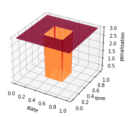
Z = eta
fig = plt.figure()
ax = plt.axes(projection='3d')
#ax.contour3D(X, Y, Z, 50, cmap='binary')
ax.plot_surface(X, Y, Z, rstride=1, cstride=1, cmap='YlOrRd', edgecolor='none')
#ax.plot_wireframe(X, Y, Z, rstride=1, cstride=1, cmap='viridis', edgecolor='none')
ax.set_xlabel('state')
ax.set_ylabel('time')
ax.set_zlabel('penalisation')
plt.show()
X, Y = np.meshgrid(y, t)
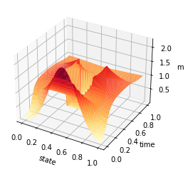
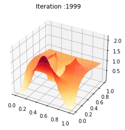
Z = av_m_1
fig = plt.figure()
ax = plt.axes(projection='3d')
#ax.contour3D(X, Y, Z, 50, cmap='YlOrRd')
ax.plot_surface(X, Y, Z, rstride=1, cstride=1, cmap='YlOrRd', edgecolor='none')
#ax.plot_wireframe(X, Y, Z, rstride=1, cstride=1, cmap='v£iridis', edgecolor='none')
ax.set_xlabel('state')
ax.set_ylabel('time')
ax.set_zlabel('m')
plt.savefig('chambolle_pock_bregman_constraint_mfg_m.png',dpi=500, bbox_inches='tight')
X, Y = np.meshgrid(t, y)
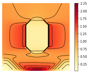
Z = av_m_1
minm = np.min(m_1_bar)
maxm = np.max(m_1_bar)
levels = np.linspace(minm,maxm,10)
fig, ax = plt.subplots()
im = ax.imshow(Z, interpolation='bilinear', origin='lower',
cmap='YlOrRd')
plt.axis('off')
CS = ax.contour(Z,levels, origin='lower', colors='black',
linewidths=1)
CBI = fig.colorbar(im)
plt.savefig('chambolle_pock_bregman_constraint_mfg_m_contour.png', dpi=500, bbox_inches='tight')
t = np.linspace(0, 1, T)
y = np.linspace(0, 1, n)
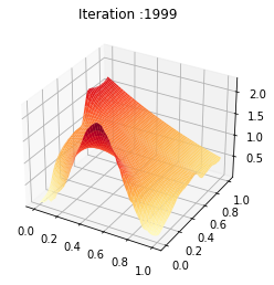
Nb_im = 2000
X, Y = np.meshgrid(y, t)
Z = ev_m[:Nb_im]
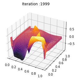
def update_plot(frame_number, zarray, plot):
plot[0].remove()
plt.title('Iteration :%s'%frame_number)
plot[0] = ax.plot_surface(X, Y, Z[frame_number,:,:], cmap="YlOrRd",edgecolor='none')
fig = plt.figure()
ax = fig.add_subplot(111, projection='3d')
fps = 100
plot = [ax.plot_surface(X, Y, Z[0,:,:], rstride=1, cstride=1)]
ani = animation.FuncAnimation(fig, update_plot, Nb_im, fargs=(Z, plot), interval=2000/fps)
ani.save('chambolle_pock_bregman_constraint_mfg_m_convergence.mp4',writer='ffmpeg',fps=fps)
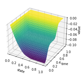
X, Y = np.meshgrid(y, t)
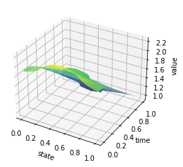
Z = U
fig = plt.figure()
ax = plt.axes(projection='3d')
#ax.contour3D(X, Y, Z, 50, cmap='magma')
ax.plot_surface(X, Y, Z, rstride=1, cstride=1, cmap='viridis', edgecolor='none')
#ax.plot_wireframe(X, Y, Z, rstride=1, cstride=1, cmap='viridis', edgecolor='none')
ax.set_xlabel('state')
ax.set_ylabel('time')
ax.set_zlabel('value')
plt.savefig('chambolle_pock_bregman_constraint_mfg_u.png',dpi=500, bbox_inches='tight')
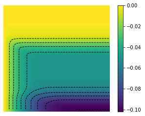
X, Y = np.meshgrid(t, y)
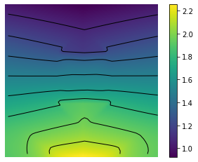
Z = U
minu = np.min(U)
maxu = np.max(U)
levels = np.linspace(minu,maxu,10)
fig, ax = plt.subplots()
im = ax.imshow(Z, interpolation='bilinear', origin='lower',
cmap='viridis')
plt.axis('off')
CS = ax.contour(Z,levels, origin='lower', colors='black',
linewidths=1)
CBI = fig.colorbar(im)
plt.savefig('chambolle_pock_bregman_constraint_mfg_u_contour.png',dpi=500, bbox_inches='tight')
t = np.linspace(0, 1, T)
y = np.linspace(0, 1, n)

Nb_im = 2000
X, Y = np.meshgrid(y, t)
Z = ev_u[:Nb_im]

def update_plot(frame_number, zarray, plot):
    plot[0].remove()
    plt.title('Iteration :%s'%frame_number)
    plot[0] = ax.plot_surface(X, Y, Z[frame_number,:,:], cmap="viridis",edgecolor='none')

fig = plt.figure()
ax = fig.add_subplot(111, projection='3d')
fps = 100
plot = [ax.plot_surface(X, Y, Z[0,:,:], rstride=1, cstride=1)]
ani = animation.FuncAnimation(fig, update_plot, Nb_im, fargs=(Z, plot), interval=2000/fps)

ani.save('chambolle_pock_bregman_constraint_mfg_u_convergence.mp4',writer='ffmpeg',fps=fps)
X, Y = np.meshgrid(y, t)
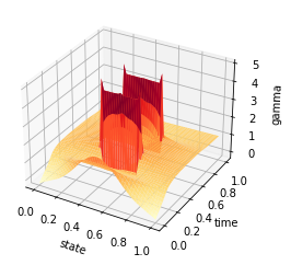
Z = av_gamma
fig = plt.figure()
ax = plt.axes(projection='3d')
#ax.contour3D(X, Y, Z, 50, cmap='binary')
ax.plot_surface(X, Y, Z, rstride=1, cstride=1, cmap='YlOrRd', edgecolor='none')
#ax.plot_wireframe(X, Y, Z, rstride=1, cstride=1, cmap='viridis', edgecolor='none')
ax.set_xlabel('state')
ax.set_ylabel('time')
ax.set_zlabel('gamma')
plt.savefig('chambolle_pock_bregman_constraint_mfg_gamma.png',dpi=500, bbox_inches='tight')
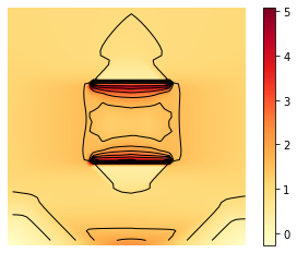
X, Y = np.meshgrid(t, y)
Z = av_gamma

mingamma = np.min(av_gamma)
maxgamma = np.max(av_gamma)
levels = np.linspace(mingamma,maxgamma,10)

fig, ax = plt.subplots()
im = ax.imshow(Z, interpolation='bilinear', origin='lower',
                cmap='YlOrRd')
plt.axis('off')
CS = ax.contour(Z,levels, origin='lower', colors='black',
                linewidths=1)
CBI = fig.colorbar(im)

plt.savefig('chambolle_pock_bregman_constraint_mfg_gamma_contour.png', dpi=500, bbox_inches='tight')
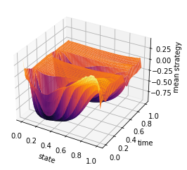
ti = np.linspace(0, 1, T-1)
y = np.linspace(0, 1, n)
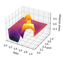
X, Y = np.meshgrid(y, ti)
Z = mean_field_strategy(Pi,T,n)
fig = plt.figure()
ax = plt.axes(projection='3d')
#ax.contour3D(X, Y, Z, 50, cmap='magma')
ax.plot_surface(X, Y, Z, rstride=1, cstride=1, cmap='inferno', edgecolor='none')
#ax.plot_wireframe(X, Y, Z, rstride=1, cstride=1, cmap='viridis', edgecolor='none')
ax.set_xlabel('state')
ax.set_ylabel('time')
ax.set_zlabel('mean strategy')
plt.savefig('chambolle_pock_bregman_constraint_mfg_mean_strategy.png', dpi=500, bbox_inches='tight')
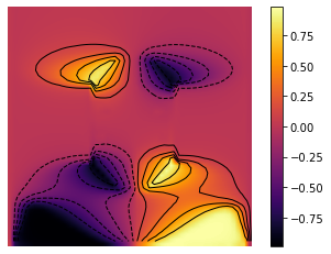
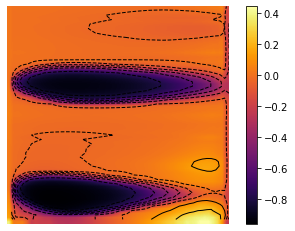
minm = np.min(Z)
maxm = np.max(Z)
levels = np.linspace(minm,maxm,10)

fig, ax = plt.subplots()
im = ax.imshow(Z, interpolation='bilinear', origin='lower',
                cmap='inferno')
plt.axis('off')
CS = ax.contour(Z,levels, origin='lower', colors='black',
                linewidths=1)
CBI = fig.colorbar(im)

plt.savefig('chambolle_pock_bregman_constraint_mfg_mean_strategy_contour.png', dpi=500, bbox_inches='tight')
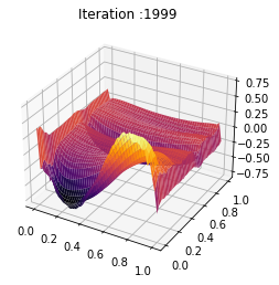
t = np.linspace(0, 1, T-1)
y = np.linspace(0, 1, n)

Nb_im = 2000
X, Y = np.meshgrid(y, t)
Z = ev_m_s[:Nb_im]

def update_plot(frame_number, zarray, plot):
    plot[0].remove()
    plt.title('Iteration :%s'%frame_number)
    plot[0] = ax.plot_surface(X, Y, Z[frame_number,:,:], cmap="inferno",edgecolor='none')

fig = plt.figure()
ax = fig.add_subplot(111, projection='3d')
fps = 100
plot = [ax.plot_surface(X, Y, Z[0,:,:], rstride=1, cstride=1)]
ani = animation.FuncAnimation(fig, update_plot, Nb_im, fargs=(Z, plot), interval=2000/fps)

ani.save('chambolle_pock_bregman_constraint_mfg_mean_strategy_convergence.mp4',writer='ffmpeg',fps=fps)
MFGC
T = 50
n = 50

alpha = alpha_cost(T,n)


L = norm_A(alpha,n,T)
sigma = 1/L
tau = 1/L
theta = 1
Dmin = -2
Dmax = 0

beta = displacement_cost(T,n)

nu = np.zeros((T,n))
eta = np.zeros((T,n))

D_0 = 1/2
Db = reference_demand(T)*2

m_0 = initial_mass(n)
var_m_1 = np.zeros((T,n)) + 1
var_m_2 = var_m_1
var_w = np.zeros((T-1,n,n)) + 1
var_D = Db

P = np.random.rand(T-1)
u = np.random.rand(T,n)
gamma = np.zeros((T,n))

(m_1_bar,m_2_bar,w_bar,D_bar) = (var_m_1,var_m_2,var_w,var_D)

(av_m_1,av_m_2,av_w,av_D,av_u,av_gamma,av_P) = (m_1_bar,m_2_bar,w_bar,D_bar,u,gamma,P)

print(tau)
0.008112138513416675
N = 10000
mfg_error = np.zeros((N,5))
ev_m_s = np.zeros((N,T-1,n))
ev_m = np.zeros((N,T,n))
ev_u = np.zeros((N,T,n))

start = time.time()
for i in range(N):
    print(round(i/N*100, 2),"              \r",end = '')
    P = prox_P(P,D_bar,w_bar,T,n,sigma,alpha)
    u = prox_u(u,m_1_bar,w_bar,m_0,sigma,T,n)
    gamma = prox_gamma(gamma,m_1_bar,m_2_bar,sigma)
    (m_1,m_2,w,D) = (var_m_1,var_m_2,var_w,var_D)
    var_D = D_prox_quad(D,P,T,n,tau,alpha,Db,D_0,Dmin,Dmax)
    (var_m_1,var_w) = m_1_w_proj(P,gamma,u,m_1,w,T,n,tau,alpha,beta)
    var_m_2 = m_2 + tau*gamma
    (m_1_bar,m_2_bar,w_bar,D_bar) = relax(var_m_1,var_m_2,var_w,var_D,m_1,m_2,w,D,theta)


    (av_m_1,av_m_2,av_w,av_D,av_u,av_gamma,av_P) = ergodic(var_m_1,var_m_2,var_w,var_D,u,gamma,P,av_m_1,av_m_2,av_w,av_D,av_u,av_gamma,av_P,i)
    (U,Pi) = d_p_mapping(av_m_1,av_w,av_gamma,av_P,alpha,beta,T,n,tol = 1e-4,mfg=0)
    mfg_error[i] = np.array(verification(av_P,U,av_gamma,av_m_1,Pi,av_w,T,n,beta,nu,m_0,alpha,Db,Dmin,Dmax,eta,mfg=0))
    (ev_m_s[i],ev_m[i],ev_u[i]) = (mean_field_strategy(Pi,T,n),av_m_1,U)
    end = time.time()

print("\n execution time :",round(end-start,2), "s")
99.99
 execution time : 4393.13 s
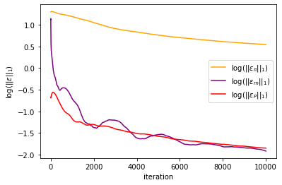
#plt.plot(np.log(mfg_error[:,0])/np.log(10), label = r'$\log(||\varepsilon_u||_1)$', color = 'blue')
plt.plot(np.log(mfg_error[:,1])/np.log(10), label = r'$\log(||\varepsilon_\pi||_1)$', color = 'orange')
plt.plot(np.log(mfg_error[:,2])/np.log(10), label = r'$\log(||\varepsilon_m||_1)$', color = 'purple')
#plt.plot(np.log(mfg_error[:,4])/np.log(10), label = r'$\log(||\varepsilon_{\gamma}||_1)$', color = 'green')
plt.plot(np.log(mfg_error[:,3])/np.log(10), label = r'$\log(||\varepsilon_P||_1)$', color = 'red')
plt.xlabel('iteration')
plt.ylabel(r'$\log(||\varepsilon||_1)$')
plt.legend()
plt.savefig('chambolle_pock_bregman_constraint_mfgc_error.png', dpi=500, bbox_inches='tight')
plt.show()
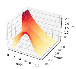
t = np.linspace(0, 1, T)
y = np.linspace(0, 1, n)

X, Y = np.meshgrid(y, t)
Z = av_m_1

fig = plt.figure()
ax = plt.axes(projection='3d')
#ax.contour3D(X, Y, Z, 50, cmap='binary')
ax.plot_surface(X, Y, Z, rstride=1, cstride=1, cmap='YlOrRd', edgecolor='none')
#ax.plot_wireframe(X, Y, Z, rstride=1, cstride=1, cmap='v£iridis', edgecolor='none')
ax.set_xlabel('state')
ax.set_ylabel('time')
ax.set_zlabel('m')

plt.savefig('chambolle_pock_bregman_constraint_mfgc_m.png', dpi=500, bbox_inches='tight')
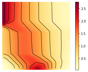
X, Y = np.meshgrid(t, y)
Z = av_m_1

minm = np.min(m_1_bar)
maxm = np.max(m_1_bar)
levels = np.linspace(minm,maxm,10)

fig, ax = plt.subplots()
im = ax.imshow(Z, interpolation='bilinear', origin='lower',
                cmap='YlOrRd')
plt.axis('off')
CS = ax.contour(Z,levels, origin='lower', colors='black',
                linewidths=1)
CBI = fig.colorbar(im)


plt.savefig('chambolle_pock_bregman_constraint_mfgc_m_contour.png', dpi=500, bbox_inches='tight')
t = np.linspace(0, 1, T)
y = np.linspace(0, 1, n)

Nb_im = 2000
X, Y = np.meshgrid(y, t)
Z = ev_m[:Nb_im]

def update_plot(frame_number, zarray, plot):
    plot[0].remove()
    plt.title('Iteration :%s'%frame_number)
    plot[0] = ax.plot_surface(X, Y, Z[frame_number,:,:], cmap="YlOrRd",edgecolor='none')

fig = plt.figure()
ax = fig.add_subplot(111, projection='3d')
fps = 100
plot = [ax.plot_surface(X, Y, Z[0,:,:], rstride=1, cstride=1)]
ani = animation.FuncAnimation(fig, update_plot, Nb_im, fargs=(Z, plot), interval=2000/fps)

ani.save('chambolle_pock_bregman_constraint_mfgc_m_convergence.mp4',writer='ffmpeg',fps=fps)
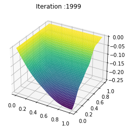
X, Y = np.meshgrid(y, t)
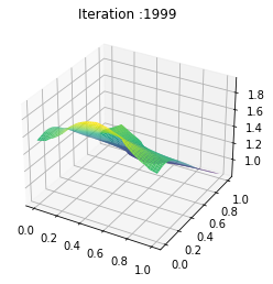
Z = U
fig = plt.figure()
ax = plt.axes(projection='3d')
#ax.contour3D(X, Y, Z, 50, cmap='magma')
ax.plot_surface(X, Y, Z, rstride=1, cstride=1, cmap='viridis', edgecolor='none')
#ax.plot_wireframe(X, Y, Z, rstride=1, cstride=1, cmap='viridis', edgecolor='none')
ax.set_xlabel('state')
ax.set_ylabel('time')
ax.set_zlabel('value')
plt.savefig('chambolle_pock_bregman_constraint_mfgc_u.png', dpi=500, bbox_inches='tight')
X, Y = np.meshgrid(t, y)
Z = U
minu = np.min(U)
maxu = np.max(U)
levels = np.linspace(minu,maxu,10)

fig, ax = plt.subplots()
im = ax.imshow(Z, interpolation='bilinear', origin='lower',
                cmap='viridis')

plt.axis('off')
CS = ax.contour(Z,levels, origin='lower', colors='black',
                linewidths=1)
CBI = fig.colorbar(im)

plt.savefig('chambolle_pock_bregman_constraint_mfgc_u_contour.png',dpi=500, bbox_inches='tight')
t = np.linspace(0, 1, T)
y = np.linspace(0, 1, n)

Nb_im = 2000
X, Y = np.meshgrid(y, t)
Z = ev_u[:Nb_im]

def update_plot(frame_number, zarray, plot):
    plot[0].remove()
    plt.title('Iteration :%s'%frame_number)
    plot[0] = ax.plot_surface(X, Y, Z[frame_number,:,:], cmap="viridis",edgecolor='none')

fig = plt.figure()
ax = fig.add_subplot(111, projection='3d')
fps = 100
plot = [ax.plot_surface(X, Y, Z[0,:,:], rstride=1, cstride=1)]
ani = animation.FuncAnimation(fig, update_plot, Nb_im, fargs=(Z, plot), interval=2000/fps)

ani.save('chambolle_pock_bregman_constraint_mfgc_u_convergence.mp4',writer='ffmpeg',fps=fps)
ti = np.linspace(0, 1, T-1)
y = np.linspace(0, 1, n)

X, Y = np.meshgrid(y, ti)
Z = mean_field_strategy(Pi,T,n)

fig = plt.figure()
ax = plt.axes(projection='3d')
#ax.contour3D(X, Y, Z, 50, cmap='magma')
ax.plot_surface(X, Y, Z, rstride=1, cstride=1, cmap='inferno', edgecolor='none')
#ax.plot_wireframe(X, Y, Z, rstride=1, cstride=1, cmap='viridis', edgecolor='none')
ax.set_xlabel('state')
ax.set_ylabel('time')
ax.set_zlabel('mean strategy')

plt.savefig('chambolle_pock_bregman_constraint_mfgc_mean_strategy.png', dpi=500, bbox_inches='tight')
minm = np.min(Z)
maxm = np.max(Z)
levels = np.linspace(minm,maxm,10)

fig, ax = plt.subplots()
im = ax.imshow(Z, interpolation='bilinear', origin='lower',
                cmap='inferno')
plt.axis('off')
CS = ax.contour(Z,levels, origin='lower', colors='black',
                linewidths=1)
CBI = fig.colorbar(im)

plt.savefig('chambolle_pock_bregman_constraint_mfgc_mean_strategy_contour.png', dpi=500, bbox_inches='tight')
t = np.linspace(0, 1, T-1)
y = np.linspace(0, 1, n)

Nb_im = 2000
X, Y = np.meshgrid(y, t)
Z = ev_m_s[:Nb_im]

def update_plot(frame_number, zarray, plot):
    plot[0].remove()
    plt.title('Iteration :%s'%frame_number)
    plot[0] = ax.plot_surface(X, Y, Z[frame_number,:,:], cmap="inferno",edgecolor='none')

fig = plt.figure()
ax = fig.add_subplot(111, projection='3d')
fps = 100
plot = [ax.plot_surface(X, Y, Z[0,:,:], rstride=1, cstride=1)]
ani = animation.FuncAnimation(fig, update_plot, Nb_im, fargs=(Z, plot), interval=2000/fps)

ani.save('chambolle_pock_bregman_constraint_mfgc_mean_strategy_convergence.mp4',writer='ffmpeg',fps=fps)
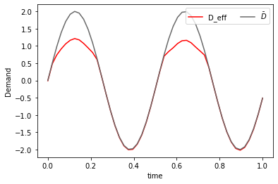
def real_demand(Db,D_0,alpha,w,T,n):
    dx = 1/n
    D_eff = np.zeros(T-1)
    for t in range(T-1):
        D_eff[t] = (np.sum(alpha[t]*w[t])*dx + Db[t])
    return(D_eff)

plt.plot(np.linspace(0,1,T-1),real_demand(Db,D_0,alpha,av_w,T,n), 'r-',label='D_eff')
plt.plot(np.linspace(0,1,T-1),Db,'dimgrey', label = r'$\bar{D}$')
plt.legend(loc='upper right',
           ncol=2)
plt.xlabel('time')
plt.ylabel('Demand')

plt.savefig('chambolle_pock_bregman_constraint_mfgc_D.png', dpi=500, bbox_inches='tight')
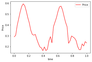
plt.plot(np.linspace(0,1,T-1),av_P, 'r-',label='Price')
plt.legend(loc='upper right',
           ncol=2)
plt.xlabel('time')
plt.ylabel('Price')

plt.savefig('chambolle_pock_bregman_constraint_mfgc_P.png', dpi=500, bbox_inches='tight')
- CP16
Antonin Chambolle and Thomas Pock. On the ergodic convergence rates of a first-order primal–dual algorithm. Mathematical Programming, 159(1):253–287, 2016.